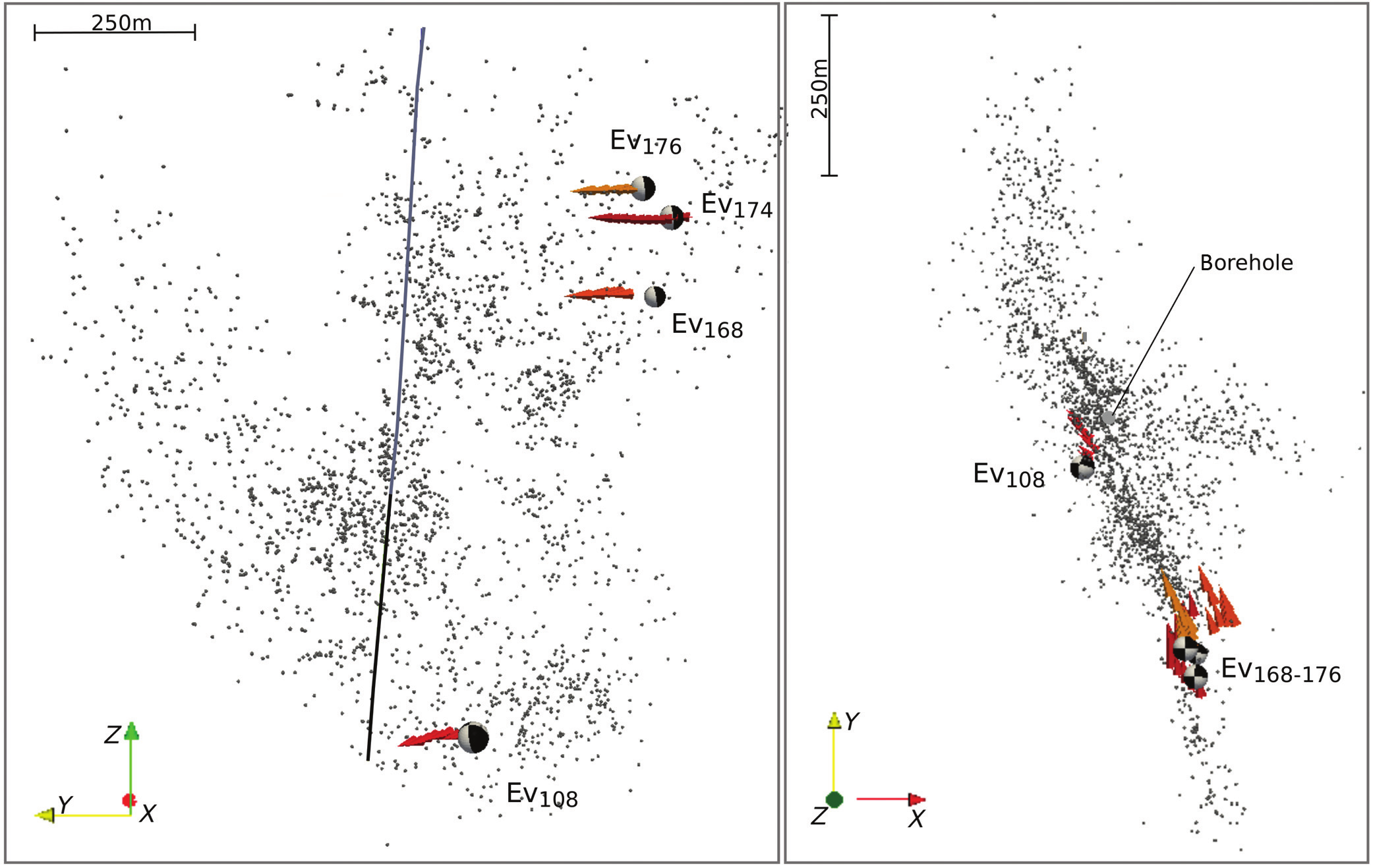
That's the result of our back-projection attempt at the Basel EGS - a geothermal power plant project was closed down because of the occurrence of a M3.4 event in 2006. The intriguing observation here was that all four M>3 events appear to rupture backward into the direction of the stress perturbation - the borehole.
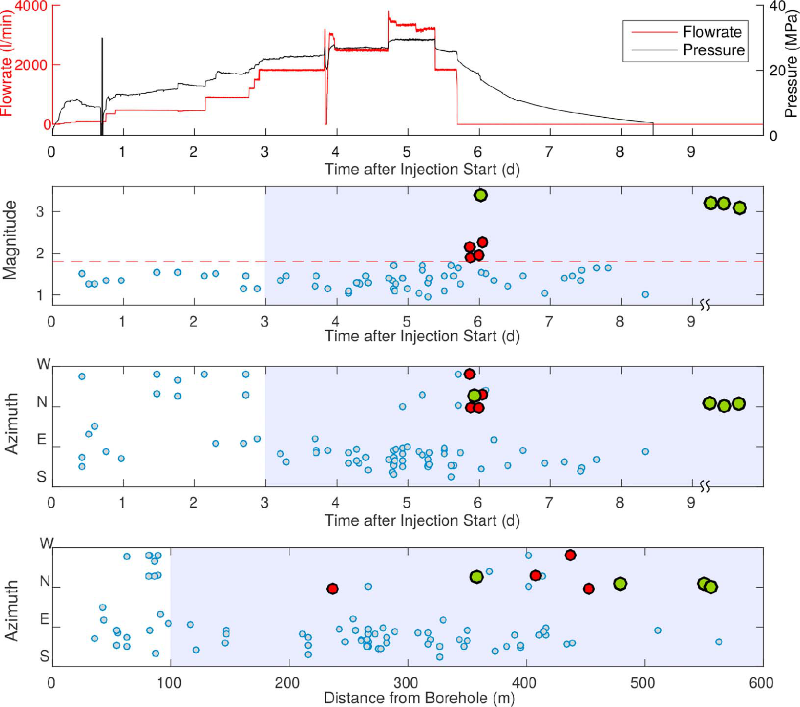
Directivity of about 80 M<3 events from the Basel EGS site in 2006. The directivity of the red events was calculated by back-projection. The directivity of the other events was obtained by fitting the peak amplitudes of their reconstructed source time functions with all possible directivity radiation patterns.
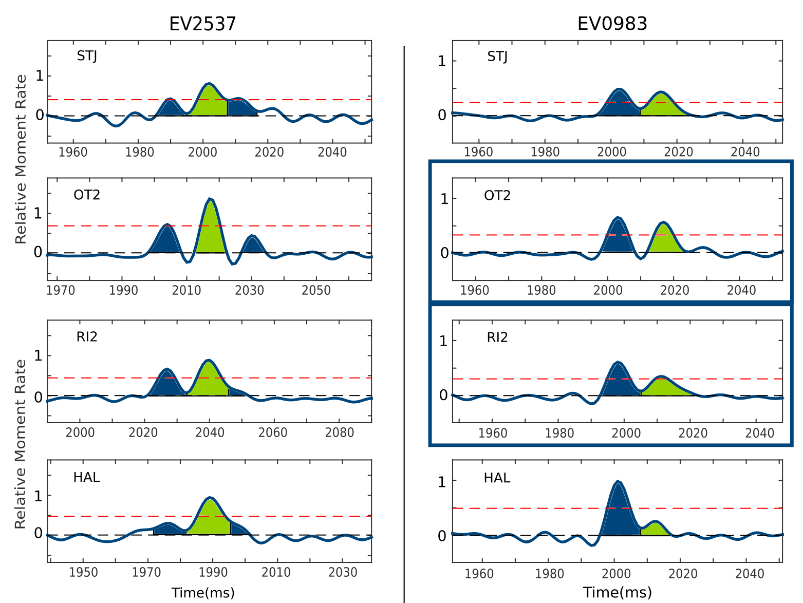
Reconstructed source-time functions for two events at four different stations showing the complexity of the rupture (not a single simple burst). The green and blue shaded peaks show different bursts of released moment and are indicative of multiple rupture phases or repeated rupture.
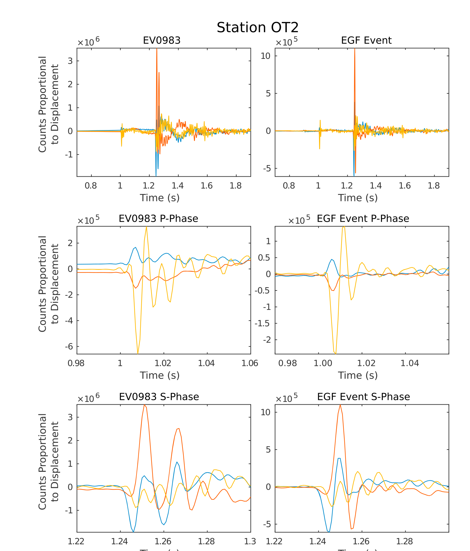
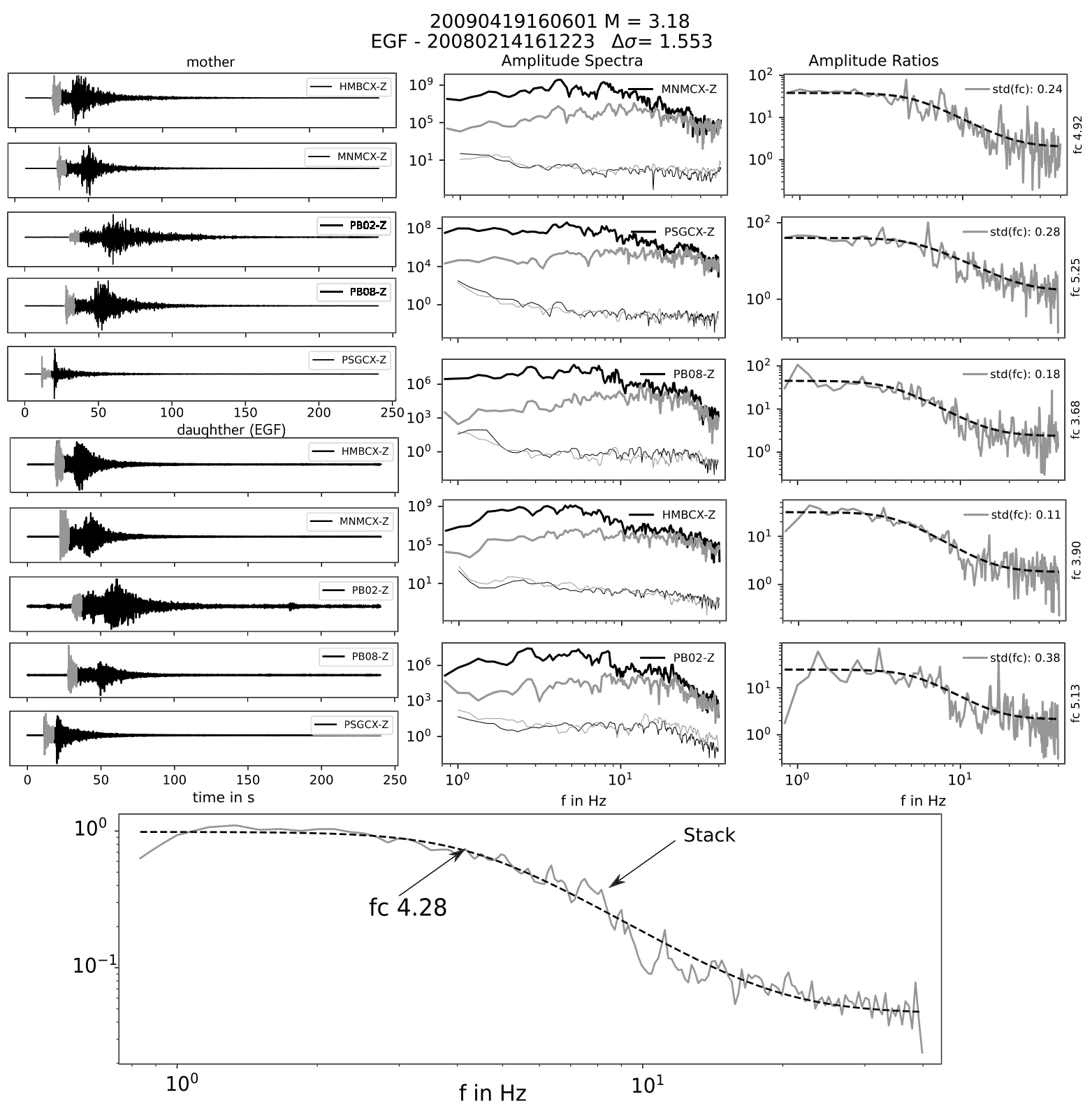
A mother and daughter event were used for spectral ratio analysis. The parent had a complex source time function. Here are her seismograms at station OT2, where the secondary event (second rupture phase) can be seen nicely in both the p- and s-phase time windows.
Spectral ratio method to extract the source spectrum of the larger event of an event pair. The obtained corner frequency can be used to estimate the source size and the stress drop.
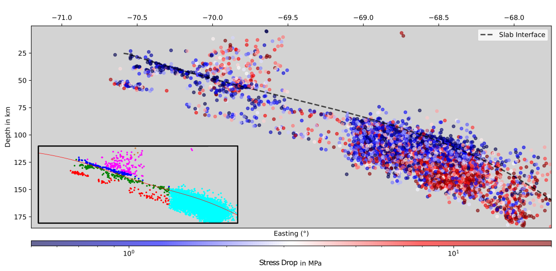
Estimated stress drops for selected earthquakes from a depth section in the northern Chilean subduction zone. Blue colors correspond to low, red colors to high stress drop. The most interesting aspect here is the slight but distinct difference of median stress drop with location. Interface stress drops are low, while upper plate stress drops are higher. The intermediate depth event stress drops show a dependence on distance from the plate surface.
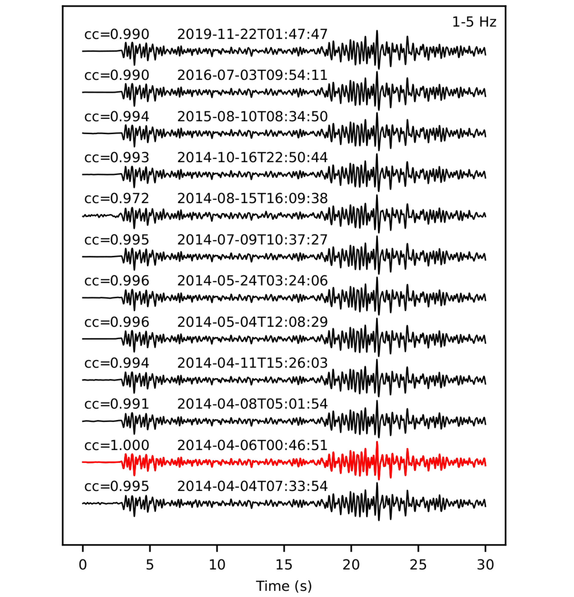
A repeating earthquake series from northern Chile. The events show an extremely high similarity in waveform, even though they occurred in different years. For this to be the case, their location, size and mechanism must be almost identical. With a filter of 1-5Hz, the naked eye cannot tell the difference between the events in this series.
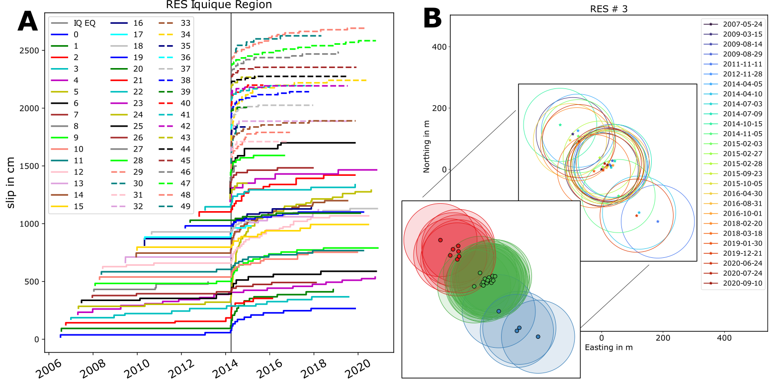
Repeating earthquakes from northern Chile. A shows the individual but cumulative displacement for 50 repeater sequences against time. The vertical black line is the 2014 MW8.1 Iquique event. B displays the high precision relocation of one repeater group demonstrating the "only" partial overlap of their estimated rupture areas.
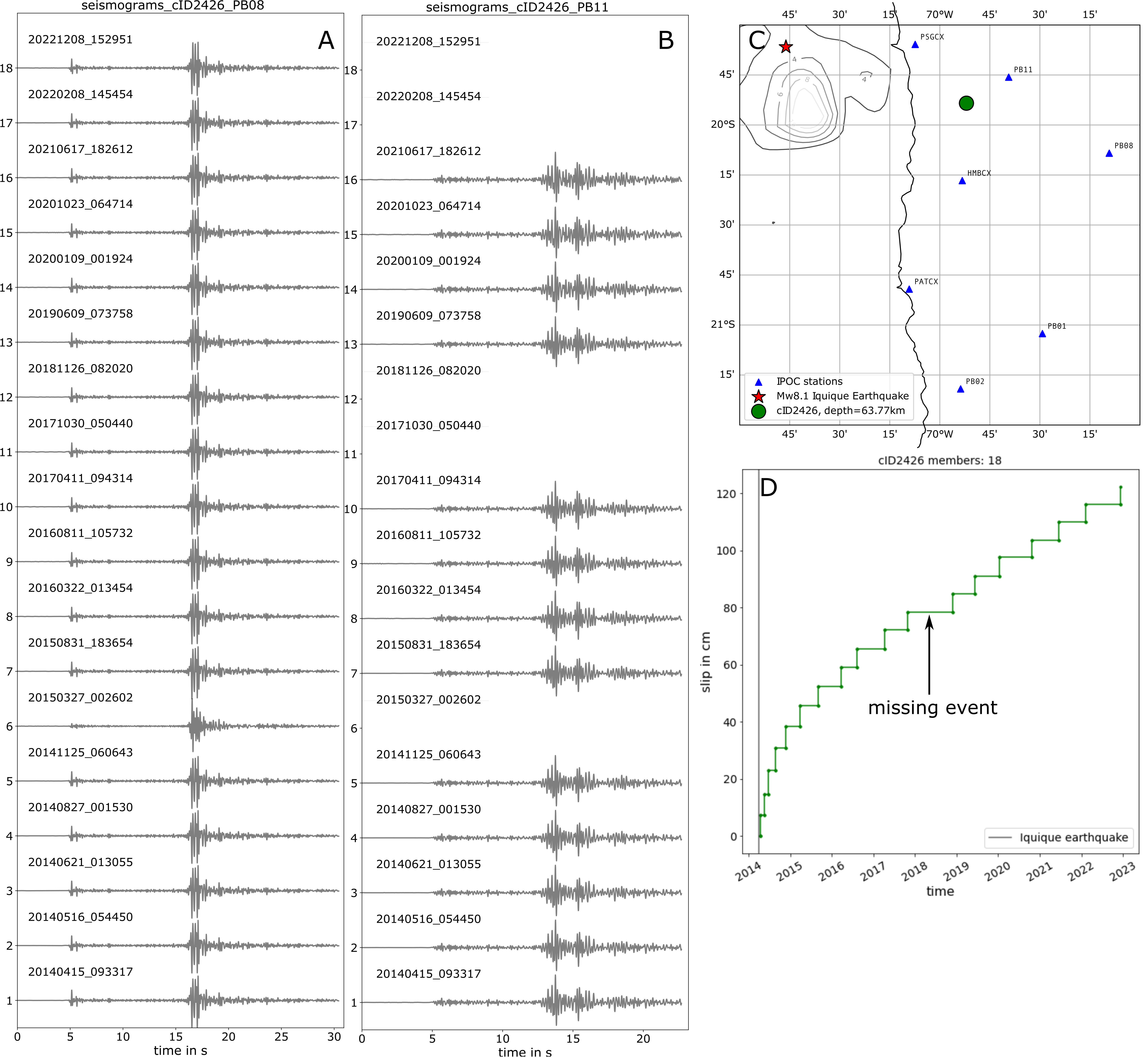
Repeating earthquake Family 2426 from northern Chile. A and B show the waveforms of the repeater sequence at two different stations. C displays the location of the series on the map. D shows the recurrence pattern (the repeats) of the repeater sequence. The vertical grey line is occurrence time of the M8.1 Iquique event. We call this series a decay type series, because the recurrence rate decays with time, illustrating the relaxation process after the large earthquake.
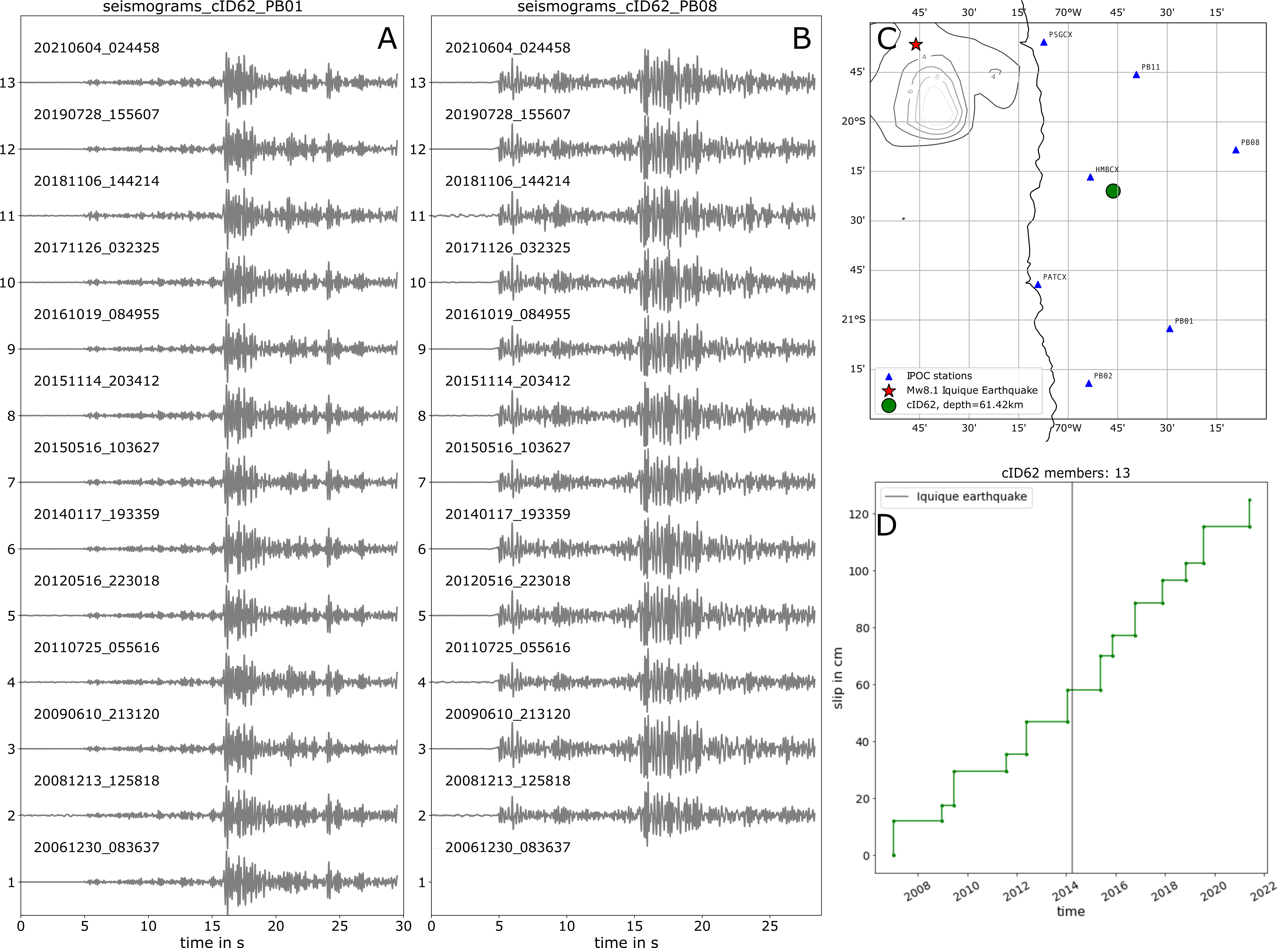
Repeating earthquake Family 62 from northern Chile. A and B again, show the waveforms of the repeater sequence at two different stations. C displays the location of the series on the map. D shows the recurrence pattern (the repeats) of the repeater sequence. The vertical grey line is occurrence time of the M8.1 Iquique event. We call this series a quasi periodic type series, because the recurrence rate is stable over a long period, with only little variation.
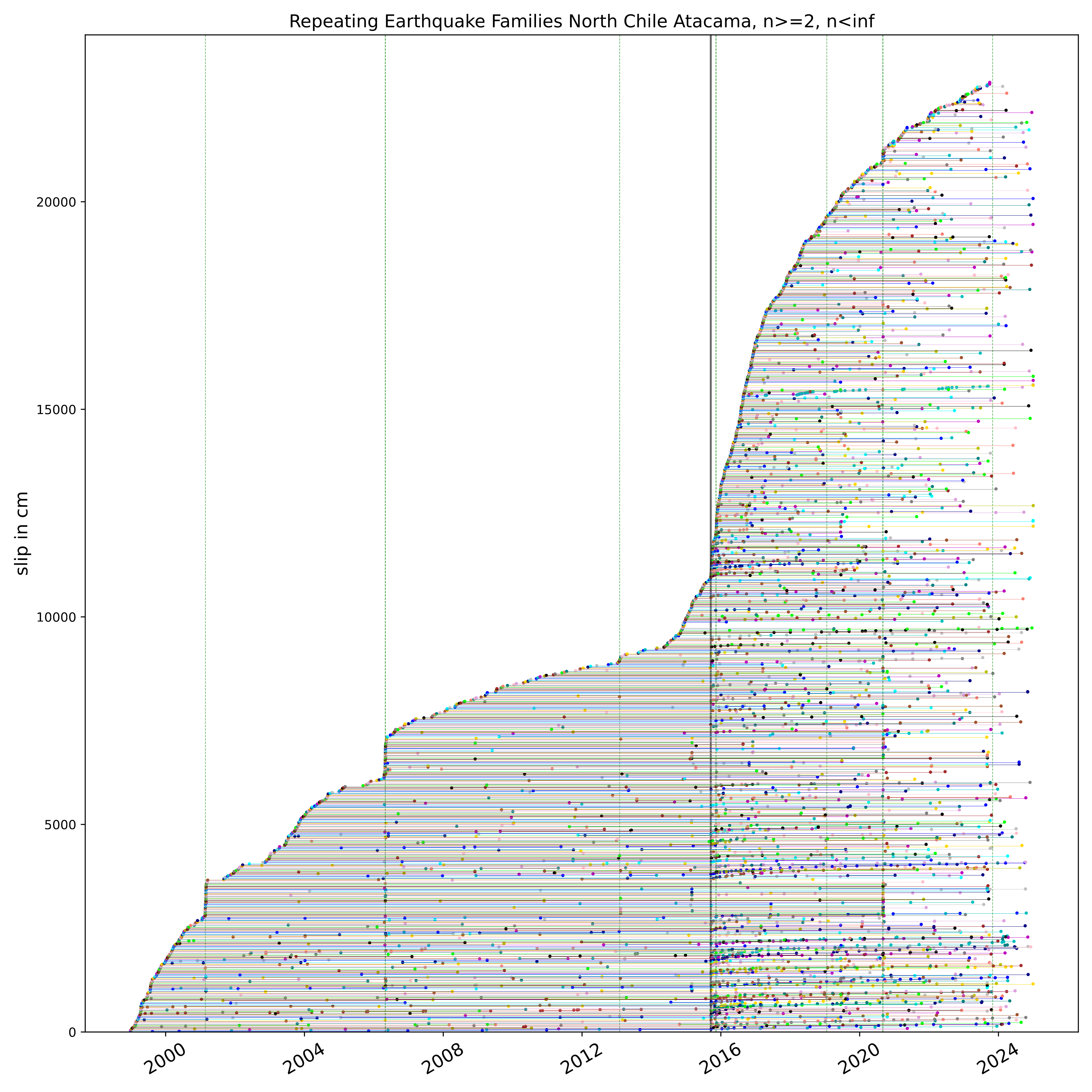
Summation plot of recurrence curves of all repeating earthquake sequences found in the Atacama Segment in North Chile. Large earthquake occurrences in the region are represented by vertical lines. The solid line is the M8.3 Illapel earthquake. Note the response of the repeaters on the large events.
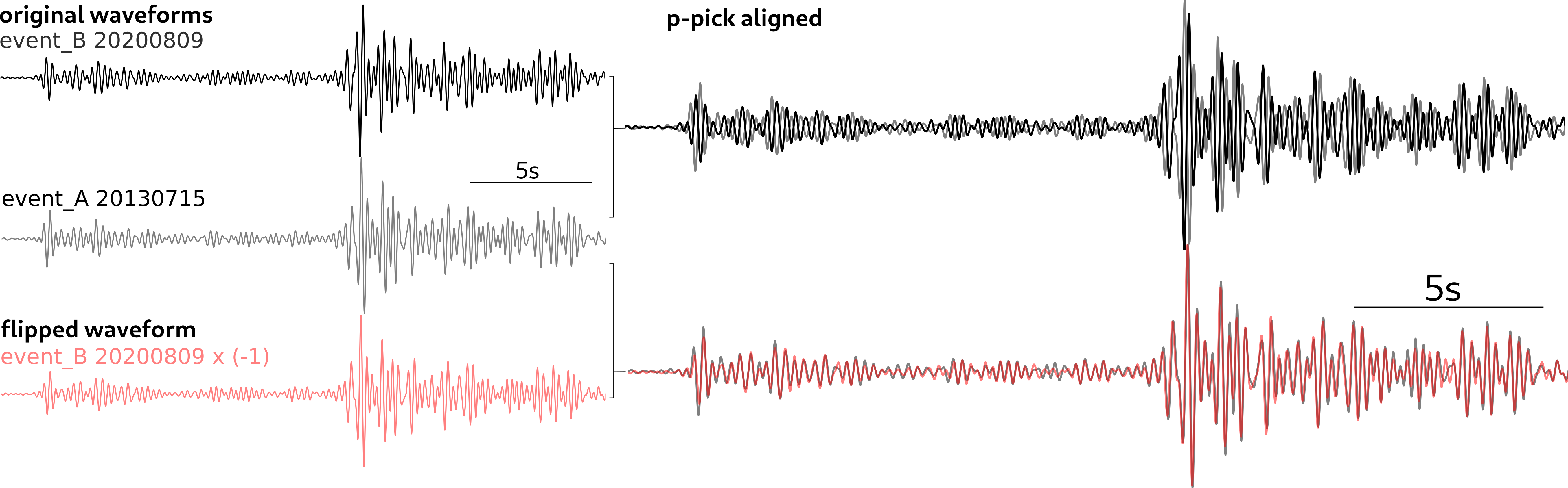
A reverse polarity event pair. Two events with almost the same seismogram, where one is the flipped version of the other. This examples stems from Northern Chile.
Events lie about 100km deep. How can we interpret such an observation? Do the event have opposite mechanisms? How is this possible at that great depth?